Introduction

Malicious software, or malware, poses a significant threat to the security and privacy of computer systems worldwide. As the frequency and sophistication of malware attacks continue to rise, the need for effective countermeasures becomes more pressing than ever. This is where malware classification comes into play. By analyzing and categorizing different types of malware, security professionals gain valuable insights that enable the development of robust defense mechanisms. One such technique is the use of Long Short-Term Memory (LSTM) models, which allows for the analysis of Windows API call sequences, unveiling patterns and behaviors that aid in identifying and combating malware. In this article, we explore the world of malware analysis using LSTM and delve into its practical applications in enhancing cybersecurity. Before we do though let’s jump into some of the terms that will be used in our experiment.

API Calls

Windows API calls, often referred to as WinAPI calls, are a set of functions and procedures provided by the Microsoft Windows operating system. These calls serve as a bridge between applications and the underlying operating system, enabling software developers to access a wide range of system functionalities. Windows API calls allow applications to perform tasks such as creating windows, interacting with files, managing processes, controlling hardware devices, and more. Each API call corresponds to a specific operation or action that can be executed by an application. These calls are essential for developers to build Windows applications that can leverage the capabilities of the operating system and interact seamlessly with its various components.

Cuckoo Sandbox

Cuckoo Sandbox is an open-source software platform designed for the dynamic analysis of suspicious files and programs. It serves as a virtualized environment where potentially malicious files, such as executables or documents, can be safely executed and monitored. Cuckoo Sandbox plays a crucial role in analyzing and understanding the behavior of these files by capturing and recording the interactions they have with the system during execution.

In the context of creating API calls, Cuckoo Sandbox monitors and logs the sequences of Windows API calls that are made by the analyzed program while running within its controlled environment. These API calls provide insights into the actions and operations the program is attempting to perform, such as file manipulation, network communication, and process management. By capturing these API calls and their associated parameters, Cuckoo Sandbox helps security researchers and analysts decipher the behavior of the program, identifying any potentially malicious or suspicious activities. This dynamic analysis approach is essential for detecting and analyzing various types of malware and cyber threats, enabling researchers to better understand their functionality and impact. They are also great for machine learning as they provide great data for models to learn from. This dynamic analysis approach is crucial in detecting and analyzing diverse forms of malware and cyber threats. It enables researchers to gain a deeper understanding of their functionality.

Dataset

Below, we will be using a ready-made data source Catak et al. (2021), that was generated using Cuckoo. Cuckoo was used to analyze more than 7000 files and create a series of Windows API calls for each file, resulting in a dataset with multiple classifications. Classification labels for each file were obtained using Virustotal. The process is illustrated in the diagram below.

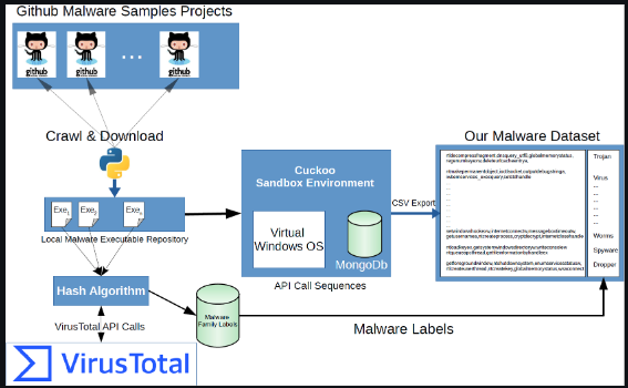
[source]

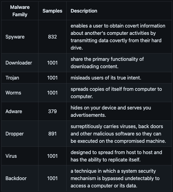
• A breakdown of the malware family labels used in the dataset and a brief description of each is shown below.

[source]

Malware Classifiers

In the realm of AI/ML, model classifiers play a crucial role in classifying various types of data, including malware. In the context of malware classification, a model classifier is an algorithm or model that learns patterns and characteristics from training data to categorize or label new instances of malware, and that’s exactly what we’ll be doing with the data shown in the previous section.

There are other classifier types but two of the most popular are single classification models and multi classification models.

1. Single-classification models aka binary models are designed to classify malware instances into a single predefined class or category. For example, a single-classification model for the trojan family would predict if a given malware file is a trojan or not. This would output a probability compared against a threshold in order to output a binary value of 1 (positive) or 0 (negative).
2. On the other hand, multi-classification models can categorize malware instances into multiple classes simultaneously. They can handle scenarios where malware samples may belong to more than one category. For instance, a multi-classification model can identify malware that is adware, spyware, or a combination of different malware types. These models provide multiple labels or probabilities for belonging to various classes.

After looking at our dataset it may appear that multi-classification is the optimal approach for this problem. However, in this experiment, we will provide support for all 8 models but will do so by creating a separate single-classification (binary) model for each. Both the binary and multi-classification models are valid solutions for addressing this problem. However, based on my research and initial experimentation, I have discovered that using multiple binary classification models as opposed to just one multi-classification model is more conducive for the model to accurately predict the classes.

What is LSTM?

Long Short-Term Memory (LSTM) is a complex subject that could warrant an entire article dedicated to explaining and understanding its intricacies. However, the main goal here is to provide a high-level explanation. LSTM is a type of RNN architecture that addresses the limitations found in traditional RNNs. Unlike standard RNNs, which struggle with capturing long-range dependencies and encountering vanishing gradient problems, LSTM introduces specialized memory cells to retain information over extended sequences. This incorporation of memory cells enables LSTM to preserve valuable context, preventing the loss of crucial information. In addition, LSTM incorporates gates that regulate the flow of information, including input, forget, and output gates. By controlling the information flow, LSTM can selectively remember or forget past information, making it ideal for tasks that require retaining relevant context over prolonged periods.

Why LSTM?

There are several ways to create malware classifiers using API call data from analyzed files. One popular approach is to use non-deep learning machine learning models like Random Forests and perform simple frequency analysis on the API calls. This method has yielded good results in other experiments. However, because of the simplicity of this model, it fails to capture the temporal nature of the sequence data in the API calls. For instance, if one malware file is represented by the sequence A, B, C, A, B, C, and another malware file is represented by the sequence C, C, A, A, B, B, both files would be treated as the same by the model because the frequency count is the same between the files (i.e. [A:2, B:2, C:2]). However, within these sequences, there could be distinct insights about a particular family of malware. Using a model that recognizes this temporal aspect could be crucial for achieving optimal results.

This is where models such as LSTM and RNN come into play. They are both excellent choices when dealing with time-series or sequential data, like the problem at hand. However, unlike traditional RNNs, LSTMs are capable of capturing long-range dependencies within sequences, making them highly proficient at retaining information across multiple time steps. Focusing on specific parts of the sequence is what makes it a valuable model for malware research. Detecting specific subsequences within a longer sequence can be decisive in determining whether a file belongs to a particular malware family. This model has already proven highly effective in various text sentiment applications, and from experimenting and reading related academic research I believe it will be effective in malware research as well.

Okay, we’re done with all the prerequisites. Now let’s jump to the code!

Loading The Dataset

First, we’ll begin with loading the data. To do this, we need two main components: the data obtained from API calls and the corresponding labels.

# create df_x and df_y from the api calls and the label data
df_x = pd.read_csv("data/all_call_data.txt", header=None)
df_y = pd.read_csv("data/all_labels.csv", header=None)

Pre-Processing

We then perform some simple statistical gathering in the code snippet below. Later on, when we’re doing further encoding, and configuring the LSTM model, we will need to know the unique count number for all text, so we extract that information here. We also perform a bit of data cleansing to make sure that the elements from the data load are of the correct type.

# get the count for the total vocab
concatenated_string = ' '.join(df_x[0])
all_strings = concatenated_string.split()
unique_count = len(set(all_strings))
print("Number of unique strings:", unique_count)

# a little data cleaning to ensure all elements were of the correct string type
df_x[0] = df_x[0].apply(lambda x: x if isinstance(x, str) else str(x))

Encoding Target Data

In this section, we are preparing our target dataset, which is the categories or classes of the malware samples. To use these categories in our machine-learning model, we need to encode them as integers. We use the LabelEncoder from the scikit-learn library to accomplish this. The fit_transform method of the LabelEncoder is applied to the target variable, df_y, to convert the categories into numerical labels. The resulting encoded labels are stored in the encoded_df_y variable.

To make things easier we also make mapping dictionaries between the classes and their associated integers. These dictionaries are convenient for working with encoded labels in the analysis and transforming back to human readable results later.

# encode categories in target to use integers
label_encoder = LabelEncoder()
encoded_df_y = label_encoder.fit_transform(df_y.iloc[:, 0])

# holds the label encoding used for the datasets
label_mapping = dict(zip(label_encoder.classes_, label_encoder.transform(label_encoder.classes_)))
inversed_mapping = {v: k for k, v in label_mapping.items()}

Tokenizing and Encoding API Call Data

In this portion of the code, we are using a Tokenizer object to learn the vocabulary from the text data. The Tokenizer is a useful tool in natural language processing that helps tokenize and vectorize text data.

Furthermore, we apply padding to ensure that all sequences have the same length. This is important when feeding the data into a machine-learning model since it typically expects fixed-length input.

# using tokenizer to learn vocabulary
tokenizer = Tokenizer(num_words = unique_count, oov_token='_UNK_')
tokenizer.fit_on_texts(df_x[0])
word_index = tokenizer.word_index

# using learned vocabulary to encode words to their distinct integer value
encoded_df_x = tokenizer.texts_to_sequences(df_x[0])
padded_encoded_df_x = pad_sequences(encoded_df_x, padding='post', maxlen=max_len)

Splitting Training and Test Data

The code snippet below transforms our one-label dataset into eight separate label datasets, each representing a different family. Since each family requires its own classifier, we need a dedicated dataset for each family, with labels of either 0 or 1 indicating if a file belongs to that family or not. The following function, given a family category, iterates over each element in the dataset and assigns a value of 1 if it matches the specified label, or 0 if it does not. This function returns a binary version of the dataset specifically tailored for that family.

# this turns the multi-classification dataset into a binary one-vs-all dataset
def split_data_by_label(df, label_num):
    df_for_label = pd.DataFrame()

    for index, elem in enumerate(df):
        df_for_label.loc[index, 0] = int(elem == label_num)
    
    return df_for_label

# dictionary to hold all of the one vs all datasets
ova_datasets = {0:'', 1:'', 2:'', 3:'', 4:'', 5:'', 6:'', 7:''}

for k,v in enumerate(ova_datasets):
    ova_datasets[k] = split_data_by_label(encoded_df_y, k)

Model Creation

This code represents a function for creating a Long Short-Term Memory (LSTM) model using Keras, a popular deep-learning library. The purpose of this function is to build a neural network model so that we can easily re-use it for each family type.

I experimented with various model architectures and found that using a similar one to Octak et al. (2021) produced the best results. I made some adjustments to this architecture during my testing, which slightly improved the results. One of the modified layers in my version is the bidirectional layer shown below, which enhances the analysis of the input by considering it from both directions.

The function create_lstm_model takes three parameters: unique_count, max_len, and act_func.

• unique_count refers to the number of unique words or tokens in the text data that will be used for training the model.
• max_len represents the maximum length of input sequences, which is necessary for creating fixed-length sequences from variable-length input texts.
• act_func denotes the activation function that will be used in the model’s layers.

Inside the function, the model is constructed step by step:

1. Sequential() is used to define a sequential model, which is a linear stack of layers.
2. Embedding(unique_count, 300, input_length=max_len) creates an embedding layer that maps each word to a dense vector representation of 300 dimensions. This layer is useful for representing words in a continuous space, capturing semantic relationships between them.
3. SpatialDropout1D(0.1) is a regularization technique that randomly drops out 10% of the dimensions in the embedding layer output. This helps prevent overfitting and improves generalization.
4. LSTM(32, dropout=0.1, recurrent_dropout=0.1, return_sequences=True, activation=act_func) adds an LSTM layer with 32 memory cells. The dropout and recurrent_dropout parameters introduce dropout to the inputs and recurrent states of the LSTM, respectively. return_sequences=True ensures that the output sequence is returned rather than just the last state.
5. Bidirectional(LSTM(64, dropout=0.1, activation=act_func)) wraps the previous LSTM layer with a bidirectional wrapper. This allows the model to learn from both past and future information by processing the input sequence in both forward and backward directions.
6. Dense(128, activation=act_func) adds a fully connected layer with 128 units and the specified activation function.
7. Dropout(0.1) applies dropout regularization to the previous layer by randomly setting 10% of the input units to 0 during training.
8. Two more Dense layers with 256 and 128 units respectively, each followed by a Dropout(0.1) layer, are added.
9. Finally, Dense(1, name='out_layer', activation="sigmoid") adds the output layer with a single unit and the sigmoid activation function, which provides a value between 0 and 1. This value indicates the probability it belongs to the class.

def create_lstm_model(unique_count, max_len, act_func):
    model = Sequential()
    model.add(Embedding(800, 300, input_length=max_len))
    model.add(SpatialDropout1D(0.1))
    model.add(LSTM(32, dropout=0.1, recurrent_dropout=0.1,
                   return_sequences=True, activation=act_func))
    model.add(Bidirectional(LSTM(64, dropout=0.1, activation=act_func)))
    model.add(Dense(128, activation=act_func))
    model.add(Dropout(0.1))
    model.add(Dense(256, activation=act_func))
    model.add(Dropout(0.1))
    model.add(Dense(128, activation=act_func))
    model.add(Dropout(0.1))
    model.add(Dense(1, name='out_layer', activation="sigmoid"))
    return model

Training and Evaluating

After creating our binary datasets it’s now time to train and evaluate them. In the code snippet below, we have a function named train_and_evaluate_model that performs training and evaluation of a machine learning model for a given dataset. This function takes several arguments, including the input data frame (df_x), the target variable (binary_y), the type of malware being analyzed (malware_type), the activation function to be used in the model (activation_func), and optional parameters to enable oversampling for minority classes and plotting results to disk.

The data is then split into training, validation, and testing sets using the train_test_split function from scikit-learn. Next, the function creates a LSTM model called ova_model using the function described in the last section. It compiles the model for a specific malware family using binary cross-entropy as the loss function, the Adam optimizer, and accuracy as the metric to analyze. To prevent overfitting, early stopping is configured with a patience of 2. This ensures that the training stops if the loss does not improve for two consecutive epochs which also saves on time and resources.

In order to evaluate the performance of the model, it goes through a series of steps. First, the model is trained using a combination of training and validation data, for a total of 10 epochs. During this process, the model’s performance is measured by tracking both the loss and accuracy values for both the training and validation sets.

After the training phase is completed, the model is then tested on unseen data, referred to as the testing set. This allows for a comprehensive evaluation of the model’s effectiveness. To further assess the model’s performance, a confusion matrix is calculated.

def train_and_evaluate_model(df_x, binary_y, malware_type, activation_func, oversample=False, plot=True):
    # to help with an imbalanced data set creating an option to oversample on the minority class to create equal distributions
    if oversample:
        oversampler = RandomOverSampler()
        df_x, binary_y = oversampler.fit_resample(df_x, binary_y)

    # Split the data into training, validation, and testing sets
    X_train, X_test, y_train, y_test = train_test_split(df_x, binary_y, test_size=0.2, random_state=42)
    X_train, X_val, y_train, y_val = train_test_split(X_train, y_train, test_size=0.3, random_state=75)

    ova_model = create_lstm_model(unique_count, max_len, activation_func)
    ova_model.compile(loss='binary_crossentropy', optimizer="adam", metrics=['accuracy'])

    # Configure early stopping
    early_stopping = EarlyStopping(monitor='loss', patience=2)

    # Train and evaluate model
    history = ova_model.fit(X_train, y_train, epochs=10, batch_size=100, callbacks=[early_stopping], validation_data=(X_val, y_val), verbose=1)

    # Store training loss and accuracy
    training_loss = history.history['loss']
    training_accuracy = history.history['accuracy']
    val_loss = history.history['val_loss']
    val_accuracy = history.history['val_accuracy']

    if plot:
        # Plot training and validation loss
        plot_loss_and_accuracy(training_loss, val_loss, training_accuracy, val_accuracy, malware_type)
    
    # test on unseen data and print confusion matrix from results
    predict_labels_and_calculate_confusion_matrix(ova_model, X_test, y_test, malware_type, activation_func)

# make a new model per classifier and for each train the model
ova_models = {0:'', 1:'', 2:'', 3:'', 4:'', 5:'', 6:'', 7:''}
activation_funcs = ['tanh', 'sigmoid', 'relu', 'softsign']

for func in activation_funcs:
    for k,v in enumerate(ova_models):
        train_and_evaluate_model(padded_encoded_df_x, ova_datasets[k], inversed_mapping[k], func, True)

Results

To gain a holistic understanding, this entire process is repeated for each activation function mentioned and for every malware classifier, resulting in a total of 32 different training and test combinations. The outcomes of these combinations are then printed out and displayed for easy comparison and analysis using the code snippet below.

# plot all all classes f1 scores for both posititive and negative classifications and do it for each activation function
model_types = ['Adware', 'Backdoor', 'Downloader', 'Dropper', 'Spyware', 'Trojan', 'Virus', 'Worms']

# Statically typed values from results. TODO to generate this in a more dynamic fashion
softsign_positive_f1 = [0.97, 0.83, 0.87, 0.84, 0.82, 0.77, 0.88, 0.79]
softsign_negative_f1 = [0.97, 0.80, 0.88, 0.82, 0.79, 0.75, 0.87, 0.79]

relu_positive_f1 = [0.84, 0.73, 0.76, 0.71, 0.73, 0.68, 0.77, 0.73]
relu_negative_f1 = [0.85, 0.72, 0.79, 0.66, 0.66, 0.66, 0.73, 0.74]

sigmoid_positive_f1 = [0.88, 0.71, 0.74, 0.69, 0.70, 0.68, 0.79, 0.71]
sigmoid_negative_f1 = [0.89, 0.73, 0.79, 0.71, 0.68, 0.70, 0.83, 0.73]

tanh_positive_f1 = [0.96, 0.83, 0.87, 0.83, 0.84, 0.76, 0.86, 0.80]
tanh_negative_f1 = [0.97, 0.83, 0.85, 0.81, 0.81, 0.76, 0.88, 0.79]

x = np.arange(len(model_types))
width = 0.35

fig, axs = plt.subplots(2, 2, figsize=(10, 8))

# Plot for softsign activation function
axs[0, 0].bar(x, softsign_positive_f1, width, label='Softsign Positive')
axs[0, 0].bar(x + width, softsign_negative_f1, width, label='Softsign Negative')
axs[0, 0].set_ylabel('F1 Score')
axs[0, 0].set_title('Softsign Positive and Negative F1 Score')
axs[0, 0].set_xticks(x)
axs[0, 0].set_xticklabels(model_types, rotation=45, ha='right')
axs[0, 0].legend()

# Plot for relu activation function
axs[0, 1].bar(x, relu_positive_f1, width, label='ReLU Positive')
axs[0, 1].bar(x + width, relu_negative_f1, width, label='ReLU Negative')
axs[0, 1].set_ylabel('F1 Score')
axs[0, 1].set_title('ReLU Positive and Negative F1 Score')
axs[0, 1].set_xticks(x)
axs[0, 1].set_xticklabels(model_types, rotation=45, ha='right')
axs[0, 1].legend()

# Plot for sigmoid activation function
axs[1, 0].bar(x, sigmoid_positive_f1, width, label='Sigmoid Positive')
axs[1, 0].bar(x + width, sigmoid_negative_f1, width, label='Sigmoid Negative')
axs[1, 0].set_ylabel('F1 Score')
axs[1, 0].set_title('Sigmoid Positive and Negative F1 Score')
axs[1, 0].set_xticks(x)
axs[1, 0].set_xticklabels(model_types, rotation=45, ha='right')
axs[1, 0].legend()

# Plot for tanh activation function
axs[1, 1].bar(x, tanh_positive_f1, width, label='Tanh Positive')
axs[1, 1].bar(x + width, tanh_negative_f1, width, label='Tanh Negative')
axs[1, 1].set_ylabel('F1 Score')
axs[1, 1].set_title('Tanh Positive and Negative F1 Score')
axs[1, 1].set_xticks(x)
axs[1, 1].set_xticklabels(model_types, rotation=45, ha='right')
axs[1, 1].legend()

plt.tight_layout()
plt.show()

Quick math lesson in case you’re not aware or forgot any of the terms used in the graphs below. Precision and recall are evaluation metrics used in machine learning and artificial intelligence to assess classification models.

Precision measures the ratio of correctly predicted positive instances out of all instances predicted as positive, focusing on minimizing false positives. Recall, on the other hand, measures the ratio of correctly predicted positive instances out of all actual positive instances, emphasizing the avoidance of false negatives.

The F1 score is a metric that balances precision and recall. It is calculated as the harmonic mean of precision and recall, providing a single evaluation value. The F1 score is especially useful for imbalanced datasets, where one class dominates the other. By considering both precision and recall, the F1 score provides a balanced measure of the model’s effectiveness in handling such datasets.

F1 Score = 2 * (Precision * Recall) / (Precision + Recall)

The bar graph shown below shows the F1 scores for each class (0s and 1), and is grouped together by the activation function that was used by the model to easily compare one another.

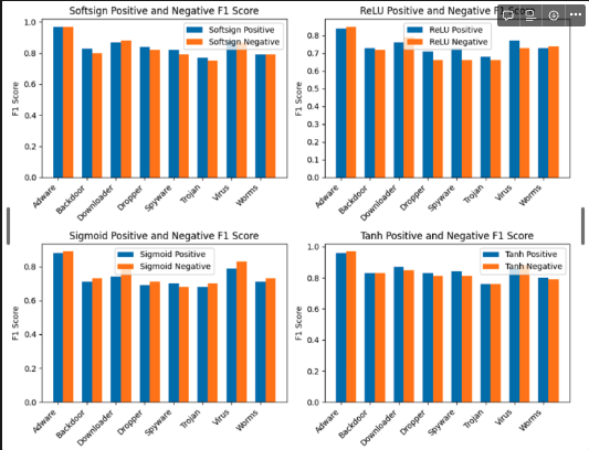
[Source: screenshot from my notebook]

Summary

One takeaway from this was the significance of the activation function utilized. Softsign and Tanh particularly excelled in producing highly efficient binary classifiers. The average F1 scores for each class using these activation functions were at least 80%.

Overall, experiments showed that LSTM is a great candidate for a prediction algorithm. I can definitely see it being used as a component in a larger data pipeline that outputs malware family types. I also learned that for some cases I prefer using multiple binary classification models instead of one multi-classification model. Although this approach will require individual attention per model and as a result could complicate maintenance, it allows for fine-tuning of specific thresholds for each family and allows models to dedicate all resources to a binary problem, which I believe as a result creates a more flexible solution and produce more accurate output.

The last point I’d like to highlight is the interesting finding that the model learned the best from Adware data, with both softsign and tanh activation functions predicting over 90% F1 scores. However, when it came to Trojan data, both activation functions had their lowest scores. This suggests that additional data and training might be necessary for the model to improve its learning capabilities. Alternatively, it could be that the current representation of the data lacks sufficient predictive power and requires some feature engineering to enable the model to extract insights and learn more effectively.

My next project aims to achieve this by utilizing both static and dynamic data, which are excellent sources for analyzing and creating classifiers using deep learning. I intend to engineer the samples by combining the data from both dynamic and static sources. This will provide a more comprehensive picture for the models to learn from, potentially leading to higher F1 scores and better insights as a result.

Conclusion

So, in conclusion, we covered various techniques for analyzing malware, and model classifiers, and discovered that LSTM models are excellent for analyzing sequential API calls derived from malware analysis. Additionally, we reviewed the results and identified areas for improvement in future projects. Thank you for reading this far and please stay tuned for more data science and malware experiments!